

This computer science problem involves algorithmic thinking and programming concepts. The solution below explains the approach, logic, and implementation step by step.
ScanSolve AI Answer
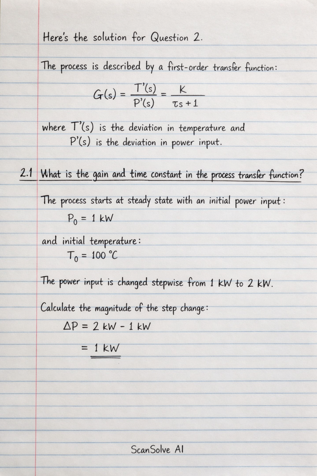
Here's the solution for Question 2. The process is described by a first-order transfer function: G(s) = (T'(s))/(P'(s)) = (K)/( s + 1) where T'(s) is the deviation in temperature and P'(s) is the deviation in power input. 2.1 What is the gain and time constant in the process transfer function? The process starts at steady state with an initial power input P_0 = 1 kW and initial temperature T_0 = 100 °C. The power input is changed stepwise from 1 kW to 2 kW. The magnitude of the step change in power input is P = 2 kW - 1 kW = 1 kW. Step 1: Determine the steady-state gain (K). After 30 minutes, the temperature stabilizes at T_ss = 500 °C. The steady-state deviation in temperature is T'_ss = T_ss - T_0 = 500 °C - 100 °C = 400 °C. For a first-order system, the steady-state gain is given by: K = Change in OutputChange in Input = T'_ss P K = 400 °C1 kW = 400 °C/kW Step 2: Determine the time constant (). For a first-order system subjected to a step change, the output response in deviation variables is: T'(t) = K P (1 - e^-t/) At t = 4 minutes, the temperature rises to T(4) = 400 °C. The deviation temperature at t=4 min is T'(4) = T(4) - T_0 = 400 °C - 100 °C = 300 °C. Substitute the known values into the equation: 300 °C = (400 °C/kW) (1 kW) (1 - e^-4/) 300 = 400 (1 - e^-4/) 0.75 = 1 - e^-4/ e^-4/ = 1 - 0.75 e^-4/ = 0.25 Take the natural logarithm of both sides: (e^-4/) = (0.25) -4/ = -1.38629 = (-4)/(-1.38629) = 2.885 min 2.2 If at another time the engineer changes the power input linearly at a rate of 0.5 kW/min, what can you say about the maximum rate of change of process temperature: When will it occur? Show your calculations in a table form. The power input changes linearly, which is a ramp input. Let the rate of change be R = 0.5 kW/min. In deviation variables, the input is P'(t) = R t. In the Laplace domain, P'(s) = (R)/(s^2). Step 1: Determine the output response in the Laplace domain. T'(s) = G(s) P'(s) = (K)/( s + 1) · (R)/(s^2) = (KR)/(s^2( s + 1)) Step 2: Derive the time-domain response for the rate of change of temperature. The inverse Laplace transform of T'(s) for a ramp input is: T'(t) = KR ( t - + e^-t/ ) To find the rate of change of process temperature, we differentiate T'(t) with respect to time: (dT'(t))/(dt) = (d)/(dt) [ KR ( t - + e^-t/ ) ] (dT'(t))/(dt) = KR ( 1 - 0 + ( -(1)/() ) e^-t/ ) (dT'(t))/(dt) = KR (1 - e^-t/) Step 3: Determine the maximum rate of change and when it occurs. The term (1 - e^-t/) starts at 0 when t=0 and increases, asymptotically approaching 1 as t → . Therefore, the maximum value of (dT'(t))/(dt) occurs as t → . The maximum rate of change is KR(1) = KR. Using the values K = 400 °C/kW and R = 0.5 kW/min: Maximum rate of change = (400 °C/kW) × (0.5 kW/min) = 200 °C/min This maximum rate of change occurs as t → . Step 4: Show calculations in a table form. We calculate the rate of change (dT'(t))/(dt) = 200 (1 - e^-t/2.885) for various time intervals. | t (min) | e^-t/ | 1 - e^-t/ | (dT'(t))/(dt) (°C/min) | | :------ | :------------ | :---------------- | :---------------------------- | | 0 | 1.000 | 0.000 | 0.0 | | 1 | 0.707 | 0.293 | 58.6 | | 2 | 0.500 | 0.500 | 100.0 | | 3 | 0.353 | 0.647 | 129.4 | | 4 | 0.250 | 0.750 | 150.0 | | 5 | 0.177 | 0.823 | 164.6 | | 10 | 0.031 | 0.969 | 193.8 | | 15 | 0.005 | 0.995 | 199.0 | | 20 | 0.001 | 0.999 | 199.8 | | | 0.000 | 1.000 | 200.0 | The table clearly shows that the rate of change of process temperature asymptotically approaches 200 °C/min as time increases. That's 2 down. 3 left today — send the next one.