
We read your photo as:
Use / VAN to calculate the optimum cost element of transportation from the transaction above.
ScanSolve AI Answer
Answer
Step-by-step solution
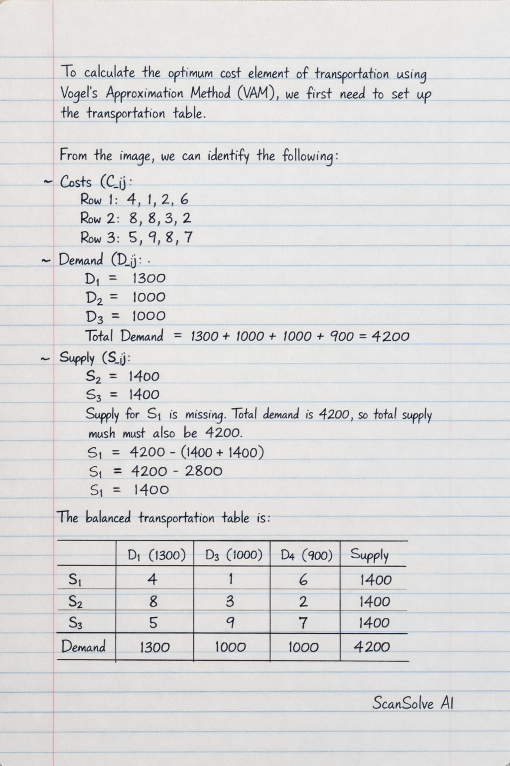
7 stepsTo calculate the optimum cost element of transportation using the Vogel's Approximation Method (VAM), we first need to set up the transportation table.
From the image, we can identify the following:
- Costs ():
- Row 1: 4, 1, 2, 6
- Row 2: 8, 8, 3, 2
- Row 3: 5, 9, 8, 7
- Demand ():
- Total Demand =
- Supply ():
- The supply for is missing. Since the total demand is 4200, we assume the total supply must also be 4200 for a balanced problem.
- Therefore, .
The balanced transportation table is:
We will now apply the VAM steps.
Calculate initial penalties.
Calculate the difference between the two lowest costs for each row and column.
Make the first allocation.
The highest penalty is 7 (Column ). In , the minimum cost is .
Allocate units to cell .
Update supply and demand: , . Column is satisfied.Recalculate penalties and make the second allocation.
The highest penalty is 4 (Column ). In , the minimum cost is .
Allocate units to cell .
Update supply and demand: , . Column is satisfied.Recalculate penalties and make the third allocation.
The highest penalty is 5 (Row ). In , the minimum cost is .
Allocate units to cell .
Update supply and demand: , . Row is satisfied.Recalculate penalties and make the fourth allocation.
The highest penalty is 6 (Column ). In , the minimum cost is .
Allocate units to cell .
Update supply and demand: , . Row is satisfied.Make the final allocations.
Only row and columns , remain.
Allocate remaining demand to .
Allocate units to cell .
Update supply and demand: , .
Allocate units to cell .
Update supply and demand: , .
All supply and demand are met.Calculate the total transportation cost.
The allocations are:
- units at cost
- units at cost
- units at cost
- units at cost
- units at cost
- units at cost
Total Cost =
Total Cost =
Total Cost = 12400
Try one yourself
A new problem that tests the same skill.
Still stuck on this one?
Ask a follow-up, and the answer starts from this question.
More Mathematics Questions
Handwritten Step-by-Step Solution
Get this as a handwritten image on WhatsApp — like a tutor wrote it for you.
Try on WhatsApp