
We read your photo as:
Answers based on engineering management
ScanSolve AI Answer
Step-by-step solution
9 stepsa and 2.b:
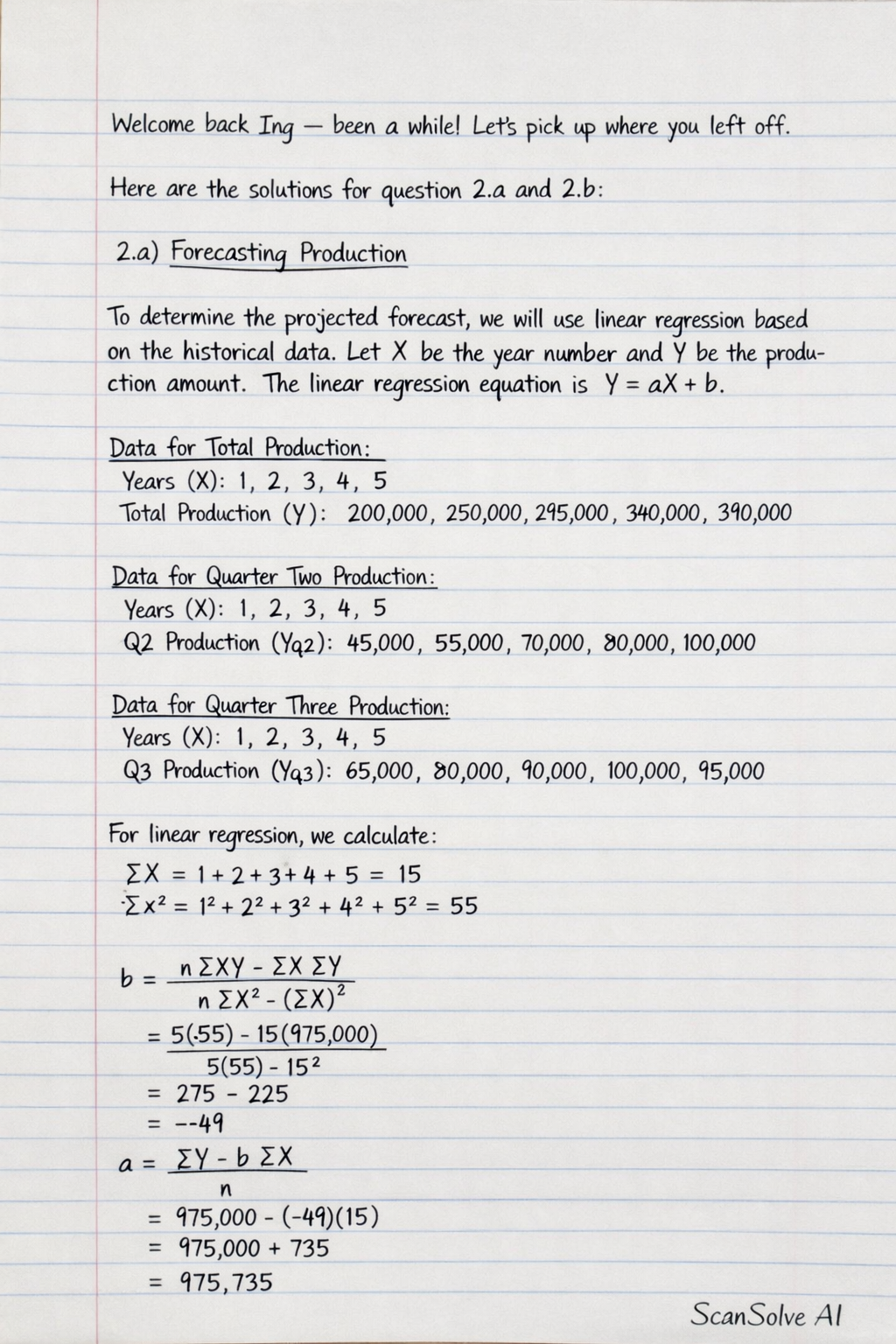
2.a) Forecasting Production
To determine the projected forecast, we will use linear regression based on the historical data. Let be the year number and be the production amount. The linear regression equation is .
-
Data for Total Production: Years (): Total Production ():
-
Data for Quarter Two Production: Years (): Quarter Two Production ():
-
Data for Quarter Three Production: Years (): Quarter Three Production ():
For linear regression, we calculate:
The slope and intercept are given by:
2.a (i) Determine the projected forecast for the seventh year.
Calculate and for total production.
Calculate the slope and intercept for total production.
The regression equation is .
Forecast for the seventh year ().
The projected forecast for the seventh year is .
2.a (ii) Determine the project production for the 2nd and 3rd quarters in the seventh year.
Calculate and for Quarter Two production.
Calculate the slope and intercept for Quarter Two.
The regression equation for Q2 is .
Forecast for Quarter Two in the seventh year ().
The projected production for the 2nd quarter in the seventh year is .
Calculate and for Quarter Three production.
Calculate the slope and intercept for Quarter Three.
The regression equation for Q3 is .
Forecast for Quarter Three in the seventh year ().
The projected production for the 3rd quarter in the seventh year is .
2.b) Define the following appraisal indicators:
-
i) Net Present Value (NPV) The Net Present Value (NPV) is the difference between the present value of cash inflows and the present value of cash outflows over a period of time. It is a capital budgeting technique used to assess the profitability of a project or investment. A positive NPV indicates that the project is expected to generate more value than its cost, making it a potentially desirable investment.
-
ii) Payback Period (PBP) The Payback Period (PBP) is the amount of time required for an investment to generate enough cash inflows to recover its initial cost. It is a simple method to evaluate the risk and liquidity of a project, with shorter payback periods generally preferred as they imply faster recovery of capital and lower risk exposure.
-
iii) Cash Flow (CF) Cash Flow refers to the net amount of cash and cash equivalents moving into and out of a business or project. It represents the actual movement of money, distinguishing it from accounting profit. Cash flow is vital for assessing a company's liquidity and solvency, and it is typically categorized into operating, investing, and financing activities.
-
Still stuck on this one?
Ask a follow-up, and the answer starts from this question.
More Business/Management Questions
Handwritten Step-by-Step Solution
Get this as a handwritten image on WhatsApp — like a tutor wrote it for you.
Try on WhatsApp