We read your photo as:

Calculate the dynamic equilibrium quantity and price for both years. Draw graphs for both years showing the supply and demand curves, the dynamic equilibria, and the producer and consumer surpluses. Calculate the total surplus for both years combined.

Economics

ScanSolve AI Answer

Answer

c

R3,741,405.46\textbf{R3,741,405.46}

Step-by-step solution

7 steps

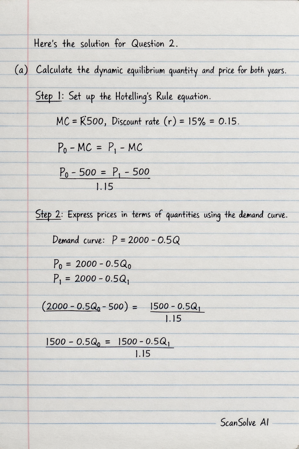
Here's the solution for Question 2.

Part a· 4 steps

Calculate the dynamic equilibrium quantity and price for both years.

  1. Set up the Hotelling's Rule equation.

    The condition for dynamic equilibrium in a finite resource market is that the present value of the net price (price minus marginal cost) is equal across periods.
    Given: Marginal Cost (MCMC) = R500, Discount rate (rr) = 15% = 0.15.

    P0−MC=P1−MC1+rP_0 - MC = \frac{P_1 - MC}{1+r} P0−500=P1−5001.15P_0 - 500 = \frac{P_1 - 500}{1.15}
  2. Express prices in terms of quantities using the demand curve.

    Demand curve: P=2000−0.5QP = 2000 - 0.5Q
    Substitute P0=2000−0.5Q0P_0 = 2000 - 0.5Q_0 and P1=2000−0.5Q1P_1 = 2000 - 0.5Q_1 into the equation from Step 1:

    (2000−0.5Q0−500)=(2000−0.5Q1−500)1.15(2000 - 0.5Q_0 - 500) = \frac{(2000 - 0.5Q_1 - 500)}{1.15} 1500−0.5Q0=1500−0.5Q11.151500 - 0.5Q_0 = \frac{1500 - 0.5Q_1}{1.15}
  3. Use the total quantity constraint to solve for quantities.

    Total quantity available: Q0+Q1=4000  ⟹  Q1=4000−Q0Q_0 + Q_1 = 4000 \implies Q_1 = 4000 - Q_0
    Substitute Q1Q_1 into the equation from Step 2:

    1500−0.5Q0=1500−0.5(4000−Q0)1.151500 - 0.5Q_0 = \frac{1500 - 0.5(4000 - Q_0)}{1.15} 1500−0.5Q0=1500−2000+0.5Q01.151500 - 0.5Q_0 = \frac{1500 - 2000 + 0.5Q_0}{1.15} 1500−0.5Q0=−500+0.5Q01.151500 - 0.5Q_0 = \frac{-500 + 0.5Q_0}{1.15}

    Multiply both sides by 1.15:

    1.15(1500−0.5Q0)=−500+0.5Q01.15(1500 - 0.5Q_0) = -500 + 0.5Q_0 1725−0.575Q0=−500+0.5Q01725 - 0.575Q_0 = -500 + 0.5Q_0 1725+500=0.5Q0+0.575Q01725 + 500 = 0.5Q_0 + 0.575Q_0 2225=1.075Q02225 = 1.075Q_0 Q0=22251.075≈2069.76744 tonnesQ_0 = \frac{2225}{1.075} \approx 2069.76744 \text{ tonnes} Q1=4000−Q0=4000−2069.76744≈1930.23256 tonnesQ_1 = 4000 - Q_0 = 4000 - 2069.76744 \approx 1930.23256 \text{ tonnes}
  4. Calculate the prices for both years.

    P0=2000−0.5Q0=2000−0.5(2069.76744)=2000−1034.88372≈R965.12P_0 = 2000 - 0.5Q_0 = 2000 - 0.5(2069.76744) = 2000 - 1034.88372 \approx R965.12 P1=2000−0.5Q1=2000−0.5(1930.23256)=2000−965.11628≈R1034.88P_1 = 2000 - 0.5Q_1 = 2000 - 0.5(1930.23256) = 2000 - 965.11628 \approx R1034.88

    The dynamic equilibrium quantities and prices are:

    • Year 0: Q0≈2069.77 tonnesQ_0 \approx \textbf{2069.77 tonnes}, P0≈R965.12P_0 \approx \textbf{R965.12}
    • Year 1: Q1≈1930.23 tonnesQ_1 \approx \textbf{1930.23 tonnes}, P1≈R1034.88P_1 \approx \textbf{R1034.88}

Part b

Draw graphs for both years showing the supply and demand curves, the dynamic equilibria, and the producer and consumer surpluses.

Since I cannot draw graphs directly, here is a description of what each graph should show:

For both Year 0 and Year 1, the graph will have Price (P) on the y-axis and Quantity (Q) on the x-axis.

  1. Demand Curve: A downward-sloping line represented by P=2000−0.5QP = 2000 - 0.5Q. This line starts at P=2000P=2000 when Q=0Q=0 and intersects the Q-axis at Q=4000Q=4000 when P=0P=0.
  2. Marginal Cost (Supply Curve): A horizontal line at P=R500P = R500. This represents the constant marginal cost of production.
  3. Dynamic Equilibrium:
    • Year 0: Mark the equilibrium point (Q0,P0)=(2069.77,965.12)(Q_0, P_0) = (2069.77, 965.12) on the demand curve.
    • Year 1: Mark the equilibrium point (Q1,P1)=(1930.23,1034.88)(Q_1, P_1) = (1930.23, 1034.88) on the demand curve.
  4. Consumer Surplus (CS): This is the area of the triangle above the equilibrium price and below the demand curve.
    • Year 0: The triangle formed by the points (0,2000)(0, 2000), (0,P0)(0, P_0), and (Q0,P0)(Q_0, P_0).
    • Year 1: The triangle formed by the points (0,2000)(0, 2000), (0,P1)(0, P_1), and (Q1,P1)(Q_1, P_1).
  5. Producer Surplus (PS): This is the area of the rectangle between the equilibrium price and the marginal cost, up to the equilibrium quantity.
    • Year 0: The rectangle formed by the points (0,MC)(0, MC), (Q0,MC)(Q_0, MC), (Q0,P0)(Q_0, P_0), and (0,P0)(0, P_0).
    • Year 1: The rectangle formed by the points (0,MC)(0, MC), (Q1,MC)(Q_1, MC), (Q1,P1)(Q_1, P_1), and (0,P1)(0, P_1).

Part c

R3,741,405.46\textbf{R3,741,405.46}

Calculate the total surplus for both years combined.

The total surplus (TS) for a given year is the area under the demand curve and above the marginal cost curve up to the equilibrium quantity.

TS=∫0Q(P(Q)−MC)dQ=∫0Q(2000−0.5Q−500)dQ=∫0Q(1500−0.5Q)dQTS = \int_0^Q (P(Q) - MC) dQ = \int_0^Q (2000 - 0.5Q - 500) dQ = \int_0^Q (1500 - 0.5Q) dQ TS=[1500Q−0.25Q2]0Q=1500Q−0.25Q2TS = \left[1500Q - 0.25Q^2\right]_0^Q = 1500Q - 0.25Q^2
  1. Calculate total surplus for Year 0 (TS0TS_0).

    Using the more precise fraction for Q0=22251.075=8900043Q_0 = \frac{2225}{1.075} = \frac{89000}{43}:

    TS0=1500(8900043)−0.25(8900043)2TS_0 = 1500 \left(\frac{89000}{43}\right) - 0.25 \left(\frac{89000}{43}\right)^2 TS0=13350000043−1479210000001849TS_0 = \frac{133500000}{43} - \frac{1}{4} \frac{7921000000}{1849} TS0=13350000043−19802500001849TS_0 = \frac{133500000}{43} - \frac{1980250000}{1849} TS0=133500000×43−19802500001849=5740500000−19802500001849=37602500001849≈R2033666.85TS_0 = \frac{133500000 \times 43 - 1980250000}{1849} = \frac{5740500000 - 1980250000}{1849} = \frac{3760250000}{1849} \approx R2033666.85
  2. Calculate total surplus for Year 1 (TS1TS_1).

    Using the more precise fraction for Q1=8300043Q_1 = \frac{83000}{43}:

    TS1=1500(8300043)−0.25(8300043)2TS_1 = 1500 \left(\frac{83000}{43}\right) - 0.25 \left(\frac{83000}{43}\right)^2 TS1=12450000043−1468890000001849TS_1 = \frac{124500000}{43} - \frac{1}{4} \frac{6889000000}{1849} TS1=12450000043−17222500001849TS_1 = \frac{124500000}{43} - \frac{1722250000}{1849} TS1=124500000×43−17222500001849=5353500000−17222500001849=36312500001849≈R1963900.00TS_1 = \frac{124500000 \times 43 - 1722250000}{1849} = \frac{5353500000 - 1722250000}{1849} = \frac{3631250000}{1849} \approx R1963900.00
  3. Calculate the present value of the total surplus for both years combined.

    PV(TS)=TS0+TS11+rPV(TS) = TS_0 + \frac{TS_1}{1+r} PV(TS)=37602500001849+363125000018491.15PV(TS) = \frac{3760250000}{1849} + \frac{\frac{3631250000}{1849}}{1.15} PV(TS)=11849(3760250000+36312500001.15)PV(TS) = \frac{1}{1849} \left( 3760250000 + \frac{3631250000}{1.15} \right) PV(TS)=11849(3760250000+3157608695.65217)PV(TS) = \frac{1}{1849} (3760250000 + 3157608695.65217) PV(TS)=6917858695.652171849≈R3741405.46PV(TS) = \frac{6917858695.65217}{1849} \approx R3741405.46

    The total surplus for both years combined (present value) is R3,741,405.46\boxed{\textbf{R3,741,405.46}}.

Was this helpful?

Try one yourself

A new problem that tests the same skill.

Still stuck on this one?

Ask a follow-up, and the answer starts from this question.

Got a different question?Ask your own question
Handwritten step-by-step solution preview

Handwritten Step-by-Step Solution

Get this as a handwritten image on WhatsApp — like a tutor wrote it for you.

Try on WhatsApp