Draw the demand and supply curves and label them D1 and S1. Mark the equilibrium price and quantity on the graph. Assume the government imposes a sales tax of K2.00 per unit supplied. Draw the new supply curve after tax and label it S2. Mark this on your graph. What is the new equilibrium price?

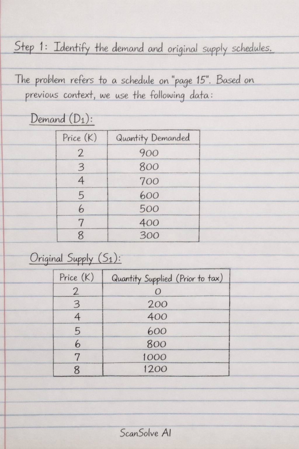
Step 1: Identify the demand and original supply schedules. The problem refers to a schedule on "page 15". Based on previous context, we use the following data: Demand (D1): | Price (K) | Quantity Demanded | |---|---| | 2 | 900 | | 3 | 800 | | 4 | 700 | | 5 | 600 | | 6 | 500 | | 7 | 400 | | 8 | 300 | Original Supply (S1): | Price (K) | Quantity Supplied (Prior to tax) | |---|---| | 2 | 0 | | 3 | 200 | | 4 | 400 | | 5 | 600 | | 6 | 800 | | 7 | 1000 | | 8 | 1200 | Step 2: Address parts a) and b) - Initial equilibrium. a) To draw the demand and supply curves (D1 and S1): • Plot the Quantity Demanded points against Price (e.g., (900, K2), (800, K3), etc.) and connect them to form the demand curve D1. • Plot the Quantity Supplied (Prior to tax) points against Price (e.g., (0, K2), (200, K3), etc.) and connect them to form the supply curve S1. b) To mark the equilibrium price and quantity on the graph: • The initial equilibrium occurs where D1 intersects S1. From the table, at a price of K5, the quantity demanded is 600 units, and the quantity supplied (S1) is also 600 units. • Mark the point (600 units, K5) on your graph as the initial equilibrium. Step 3: Address parts c) and d) - New supply curve after tax. c) The government imposes a sales tax of K2.00 per unit supplied. This means that for producers to supply any given quantity, they now require K2.00 more per unit. This shifts the supply curve upwards by K2.00. d) To draw the new supply curve (S2) after tax: • For each price P, the quantity supplied on S2 is the quantity supplied on S1 at price (P - K2). The new supply schedule (S2) is: | Price (K) | Quantity Supplied (S2, after K2 tax) | |---|---| | 2 | 0 (Qs1 at P=0) | | 3 | 0 (Qs1 at P=1) | | 4 | 0 (Qs1 at P=2) | | 5 | 200 (Qs1 at P=3) | | 6 | 400 (Qs1 at P=4) | | 7 | 600 (Qs1 at P=5) | | 8 | 800 (Qs1 at P=6) | • Plot these new points (e.g., (0, K4), (200, K5), etc.) and connect them to form the new supply curve, labeling it S2. Step 4: Address part e) - New equilibrium price. e) The new equilibrium occurs where the demand curve (D1) intersects the new supply curve (S2). • We need to find the price where Quantity Demanded (Q_D) equals Quantity Supplied after tax (Q_S2). From the tables: | Price (K) | Quantity Demanded (D1) | Quantity Supplied (S2) | |---|---|---| | 6 | 500 | 400 | | 7 | 400 | 600 | The equilibrium price is between K6 and K7. • To find the exact price, we derive the linear equations for D1 and S2. Demand curve (D1): Using points (K6, 500) and (K7, 400). Slope m_D = (400 - 500)/(7 - 6) = -100. Equation: Q_D - 500 = -100(P - 6) Q_D = -100P + 1100. Supply curve (S2): Using points (K6, 400) and (K7, 600). Slope m_S = (600 - 400)/(7 - 6) = 200. Equation: Q_S2 - 400 = 200(P - 6) Q_S2 = 200P - 800. • Set Q_D = Q_S2 to find the new equilibrium price: 1100 - 100P = 200P - 800 1100 + 800 = 200P + 100P 1900 = 300P P = (1900)/(300) = (19)/(3) P ≈ 6.33 The new equilibrium price is K(19)/(3) or approximately K6.33. That's 2 down. 3 left today — send the next one.