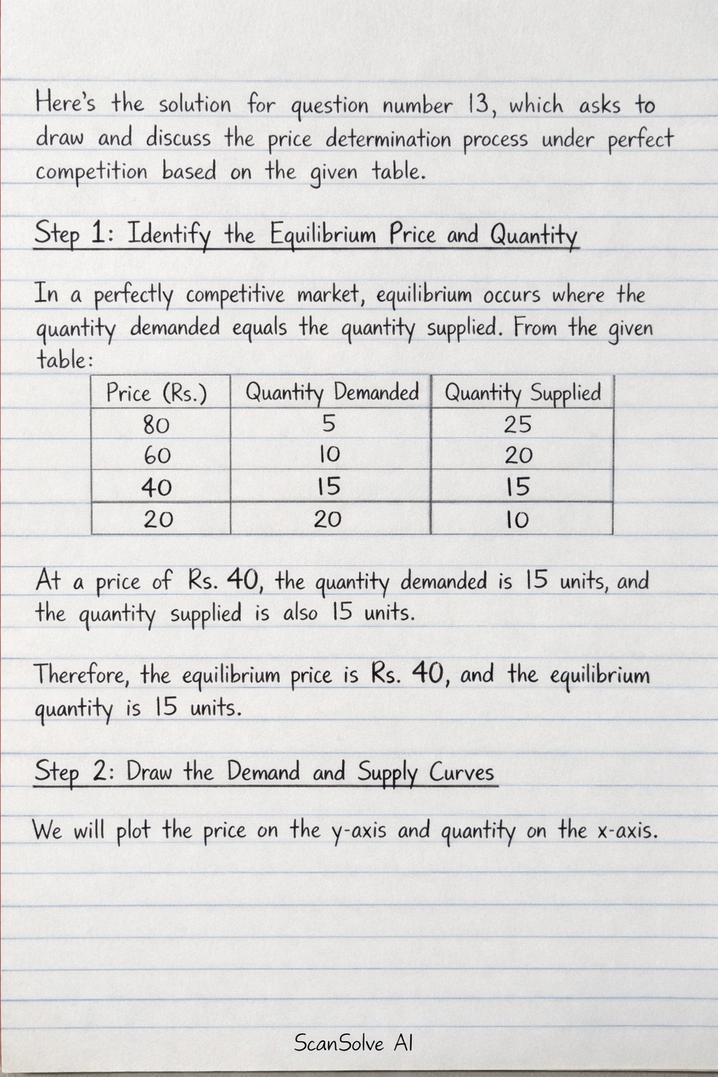
Here's the solution for question number 13, which asks to draw and discuss the price determination process under perfect competition based on the given table. Step 1: Identify the Equilibrium Price and Quantity In a perfectly competitive market, equilibrium occurs where the quantity demanded equals the quantity supplied. From the given table: | Price (Rs.) | Quantity Demanded | Quantity Supplied | | :---------- | :---------------- | :---------------- | | 80 | 5 | 25 | | 60 | 10 | 20 | | 40 | 15 | 15 | | 20 | 20 | 10 | At a price of Rs. 40, the quantity demanded is 15 units, and the quantity supplied is also 15 units. Therefore, the equilibrium price is Rs. 40, and the equilibrium quantity is 15 units. Step 2: Draw the Demand and Supply Curves We will plot the price on the y-axis and quantity on the x-axis. Demand Curve (D): Connect the points (5, 80), (10, 60), (15, 40), (20, 20). Supply Curve (S): Connect the points (25, 80), (20, 60), (15, 40), (10, 20). The graph will show the demand curve sloping downwards and the supply curve sloping upwards. They intersect at the equilibrium point. $$ \text{Graph: Price Determination under Perfect Competition} $$ $$ \begin{tikzpicture} \begin{axis}[ xlabel={Quantity}, ylabel={Price (Rs.)}, xmin=0, xmax=30, ymin=0, ymax=100, xtick={0,5,10,15,20,25}, ytick={0,20,40,60,80}, grid=both, legend pos=north west, legend style={draw=none,fill=none} ] \addplot[blue, thick, mark=*, samples=5, domain=5:20] coordinates { (5,80) (10,60) (15,40) (20,20) }; \addlegendentry{Demand (D)} \addplot[red, thick, mark=*, samples=5, domain=10:25] coordinates { (25,80) (20,60) (15,40) (10,20) }; \addlegendentry{Supply (S)} \draw[dashed] (axis cs:15,0) -- (axis cs:15,40); \draw[dashed] (axis cs:0,40) -- (axis cs:15,40); \node[below left] at (axis cs:15,0) {$Q_e=15$}; \node[above right] at (axis cs:0,40) {$P_e=40$}; \node[above right] at (axis cs:15,40) {E}; \end{axis} \end{tikzpicture} $$ Step 3: Discuss the Price Determination Process Under perfect competition, the market price and quantity are determined by the interaction of total market demand and total market supply. • The demand curve (D) shows the inverse relationship between price and quantity demanded: as price falls, quantity demanded rises. • The supply curve (S) shows the direct relationship between price and quantity supplied: as price rises, quantity supplied rises. • The equilibrium point (E) is where the demand and supply curves intersect. At this point, the quantity consumers are willing and able to buy ($Q_e$) exactly matches the quantity producers are willing and able to sell ($Q_e$). • In this specific case, the equilibrium price ($P_e$) is Rs. 40, and the equilibrium quantity ($Q_e$) is 15 units. • If the price were above equilibrium (e.g., Rs. 60), there would be a surplus (supply > demand), pushing prices down. • If the price were below equilibrium (e.g., Rs. 20), there would be a shortage (demand > supply), pushing prices up. • The market naturally adjusts to the equilibrium price and quantity where there is no pressure for the price to change. The final answer is $\boxed{\text{Equilibrium Price = Rs. 40, Equilibrium Quantity = 15 units}}$.