
We read your photo as:
Find a simple discrete model for X with E[X]=1.2 and Var(X)=2.5.
ScanSolve AI Answer
Step-by-step solution
3 stepsThe problem asks to find a simple discrete model for the number of defective items per shipment, , given and .
Analyze the properties of common discrete distributions.
-
Poisson distribution: For a Poisson distribution with parameter , and . Given and . If we use a Poisson distribution, we would need and simultaneously, which is not possible. Also, the variance (2.5) is not equal to the mean (1.2). So, a Poisson distribution is not a good fit.
-
Binomial distribution: For a binomial distribution with parameters and , and . Given and . From . From . Substitute into the variance equation: . . . Since must be between 0 and 1, a binomial distribution is not a good fit.
-
Bernoulli distribution: A Bernoulli distribution is a special case of a binomial distribution where . For a Bernoulli distribution with parameter , and . Given . This would imply , which is not possible as must be between 0 and 1. So, a Bernoulli distribution is not a good fit.
-
Consider a custom two-point distribution.
A two-point distribution assigns probabilities to two distinct values. Let these values be and with probabilities and respectively, where .
The mean is .
The variance is .Let's check option D: "Use a custom two-point distribution where or with chosen probabilities that match the sample mean and variance."
If can only take values 1 or 2, let and .
Then .
We are given .
So, .
Thus, and .Now, let's calculate the variance for this distribution:
.
.This calculated variance (0.16) does not match the given . Therefore, a two-point distribution with or is not the correct model.
Re-evaluate the options based on the problem statement.
The question asks for a "simple discrete model consistent with these estimates for internal communication (even if not uniquely correct)". This implies we are looking for the best fit among the given options, even if no option perfectly matches all properties.
Let's re-examine the options:
A. Use a Poisson distribution with parameter , since Poisson has , matching the approximate mean and variance.
This statement is incorrect because and . They are not equal, so a Poisson distribution is not a good fit.B. Use a binomial distribution with parameters and so the mean matches the observed 1.2 defects per shipment.
This is a Bernoulli distribution (). As shown in Step 1, is not a valid probability. So, this option is incorrect.C. Use a Bernoulli distribution with parameter because the mean of a Bernoulli is .
This is the same issue as option B; is not a valid probability. So, this option is incorrect.D. Use a custom two-point distribution where or with chosen probabilities that match the sample mean and variance.
As shown in Step 2, if we choose or , we can match the mean () but not the variance (). However, the option states "with chosen probabilities that match the sample mean and variance". This implies that such probabilities could exist for some two-point distribution, not necessarily restricted to or .Let's consider a general two-point distribution with values and and probabilities and .
We have two equations and four unknowns (). We need to choose and such that a valid exists.
Let's try to find and that satisfy these conditions.
From .
From .
.Let's try to solve for in terms of and :
.
Substitute this into the variance equation. This will be a complex equation.However, the question asks for the best simple discrete model.
The key observation is that ().- For a Poisson distribution, .
- For a Binomial distribution, . Since , , so . Therefore, neither Poisson nor Binomial distributions can model this data because they both have variance less than or equal to the mean.
A distribution where the variance is greater than the mean is called overdispersed.
A two-point distribution can be overdispersed.
Let take values and with probabilities and .
This can be rewritten as .
We need and .
We can choose and such that these conditions are met. For example, if we choose and :
.
.
Substitute :
.
We also have , so .
Multiply by : .
.
Then .
And .
Check: .
Check: .
So, a two-point distribution can match the given mean and variance. The specific values or mentioned in option D are just an example, and the general statement "with chosen probabilities that match the sample mean and variance" is the key.Therefore, a custom two-point distribution is the only type of distribution among the options that can accommodate .
The final answer is .
Just one more to go! Send it over.
Still stuck on this one?
Ask a follow-up, and the answer starts from this question.
More Mathematics Questions
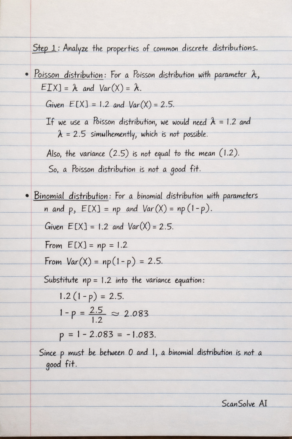
Handwritten Step-by-Step Solution
Get this as a handwritten image on WhatsApp — like a tutor wrote it for you.
Try on WhatsApp