
We read your photo as:
We want to calculate the optimum element of transportation from the transaction above.
ScanSolve AI Answer
Answer
Step-by-step solution
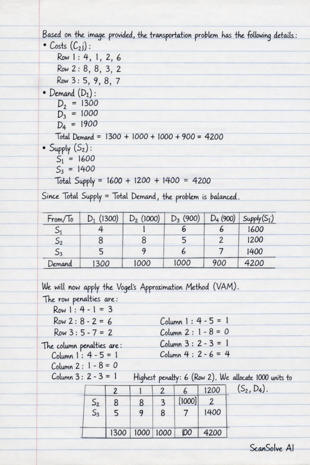
6 stepsBased on the image provided, the transportation problem has the following details:
- Costs ():
- Row 1: 4, 1, 2, 6
- Row 2: 8, 8, 3, 2
- Row 3: 5, 9, 8, 7
- Demand ():
- Total Demand =
- Supply ():
- Total Supply =
Since Total Supply = Total Demand, the problem is balanced.
The transportation table is:
We will now apply the Vogel's Approximation Method (VAM).
Calculate initial penalties and make the first allocation.
Calculate the difference between the two lowest costs for each row and column.
- Row Penalties: , ,
- Column Penalties: , , ,
The highest penalty is 7 (Column ). The minimum cost in is .
Allocate units to cell .
Update: , . Column is satisfied.Recalculate penalties and make the second allocation.
- Row Penalties: , ,
- Column Penalties: , ,
The highest penalty is 4 (Column ). The minimum cost in is .
Allocate units to cell .
Update: , . Column is satisfied.Recalculate penalties and make the third allocation.
- Row Penalties: , ,
- Column Penalties: ,
The highest penalty is 5 (Row ). The minimum cost in is .
Allocate units to cell .
Update: , . Row is satisfied.Recalculate penalties and make the fourth allocation.
- Row Penalties: ,
- Column Penalties: ,
The highest penalty is 6 (Column ). The minimum cost in is .
Allocate units to cell .
Update: , . Row is satisfied.Make the final allocations.
Only row and columns , remain.
Allocate units to cell .
Update: , .
Allocate units to cell .
Update: , .
All supply and demand are met.Calculate the total transportation cost.
The allocations are:
- units at cost
- units at cost
- units at cost
- units at cost
- units at cost
- units at cost
Total Cost =
Total Cost =
Total Cost = 12200
Try one yourself
A new problem that tests the same skill.
Still stuck on this one?
Ask a follow-up, and the answer starts from this question.
More Mathematics Questions
Handwritten Step-by-Step Solution
Get this as a handwritten image on WhatsApp — like a tutor wrote it for you.
Try on WhatsApp