Graph Construction and Analysis. The table below shows demand and supply for a Laundry Powder after sales tax. (Write your answers in the space provided below)

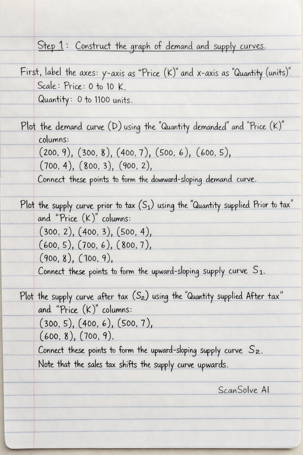
Step 1: Construct the graph of demand and supply curves. First, label the axes: the vertical axis (y-axis) as "Price (K)" and the horizontal axis (x-axis) as "Quantity (units)". Scale the Price axis from 0 to 10 K and the Quantity axis from 0 to 1100 units. Plot the demand curve (D) using the "Quantity demanded" and "Price (K)" columns: (200, 9), (300, 8), (400, 7), (500, 6), (600, 5), (700, 4), (800, 3), (900, 2). Connect these points to form the downward-sloping demand curve. Plot the supply curve prior to tax (S_1) using the "Quantity supplied Prior to tax" and "Price (K)" columns: (300, 2), (400, 3), (500, 4), (600, 5), (700, 6), (800, 7), (900, 8), (1000, 9). Connect these points to form the upward-sloping supply curve S_1. Plot the supply curve after tax (S_2) using the "Quantity supplied After tax" and "Price (K)" columns: (300, 5), (400, 6), (500, 7), (600, 8), (700, 9). Connect these points to form the upward-sloping supply curve S_2. Note that the sales tax shifts the supply curve upwards (or to the left). [scale=0.7] % Axes [->] (0,0) -- (0,10.5) node[left] Price (K); [->] (0,0) -- (11,0) node[below] Quantity (units); % Grid lines in 1,2,...,10 (,0.1) -- (,-0.1) node[below] *100; in 1,2,...,10 (0.1,) -- (-0.1,) node[left] ; % Demand Curve (D) [blue, thick] (2,9) -- (3,8) -- (4,7) -- (5,6) -- (6,5) -- (7,4) -- (8,3) -- (9,2) node[below right] D; % Supply Curve Prior to tax (S1) [red, thick] (3,2) -- (4,3) -- (5,4) -- (6,5) -- (7,6) -- (8,7) -- (9,8) -- (10,9) node[above left] S_1; % Supply Curve After tax (S2) [green!50!black, thick] (3,5) -- (4,6) -- (5,7) -- (6,8) -- (7,9) node[above left] S_2; % Equilibrium 1 (Prior to tax) [black] (6,5) circle (2pt); [dashed] (0,5) -- (6,5); [dashed] (6,0) -- (6,5); at (6.5,5.5) E_1; % Equilibrium 2 (After tax) - calculated as (450, 6.5) [black] (4.5,6.5) circle (2pt); [dashed] (0,6.5) -- (4.5,6.5); [dashed] (4.5,0) -- (4.5,6.5); at (5,7) E_2; Step 2: Analyze the equilibrium prior to tax. The equilibrium prior to tax (E_1) occurs where the demand curve (D) intersects the supply curve prior to tax (S_1). From the table, this is at a price of 5 K and a quantity of 600 units. Equilibrium Prior to Tax: Price = 5 K, Quantity = 600 units Step 3: Analyze the equilibrium after tax. The equilibrium after tax (E_2) occurs where the demand curve (D) intersects the supply curve after tax (S_2). From the table, at Price = 6 K, Quantity Demanded = 500, Quantity Supplied (After tax) = 400. At Price = 7 K, Quantity Demanded = 400, Quantity Supplied (After tax) = 500. The equilibrium is between these two points. By calculating the linear equations for demand and supply after tax, the equilibrium is found to be at a price of 6.5 K and a quantity of 450 units. Equilibrium After Tax: Price = 6.5 K, Quantity = 450 units Step 4: Explain the impact of the sales tax. The imposition of a sales tax shifts the supply curve to the left (from S_1 to S_2). This results in a higher equilibrium price (from 5 K to 6.5 K) and a lower equilibrium quantity (from 600 units to 450 units). The tax increases the cost of production for suppliers, leading them to supply less at each price level, which ultimately raises the market price for consumers and reduces the quantity traded. 4 done, 1 left today. You're doing great!