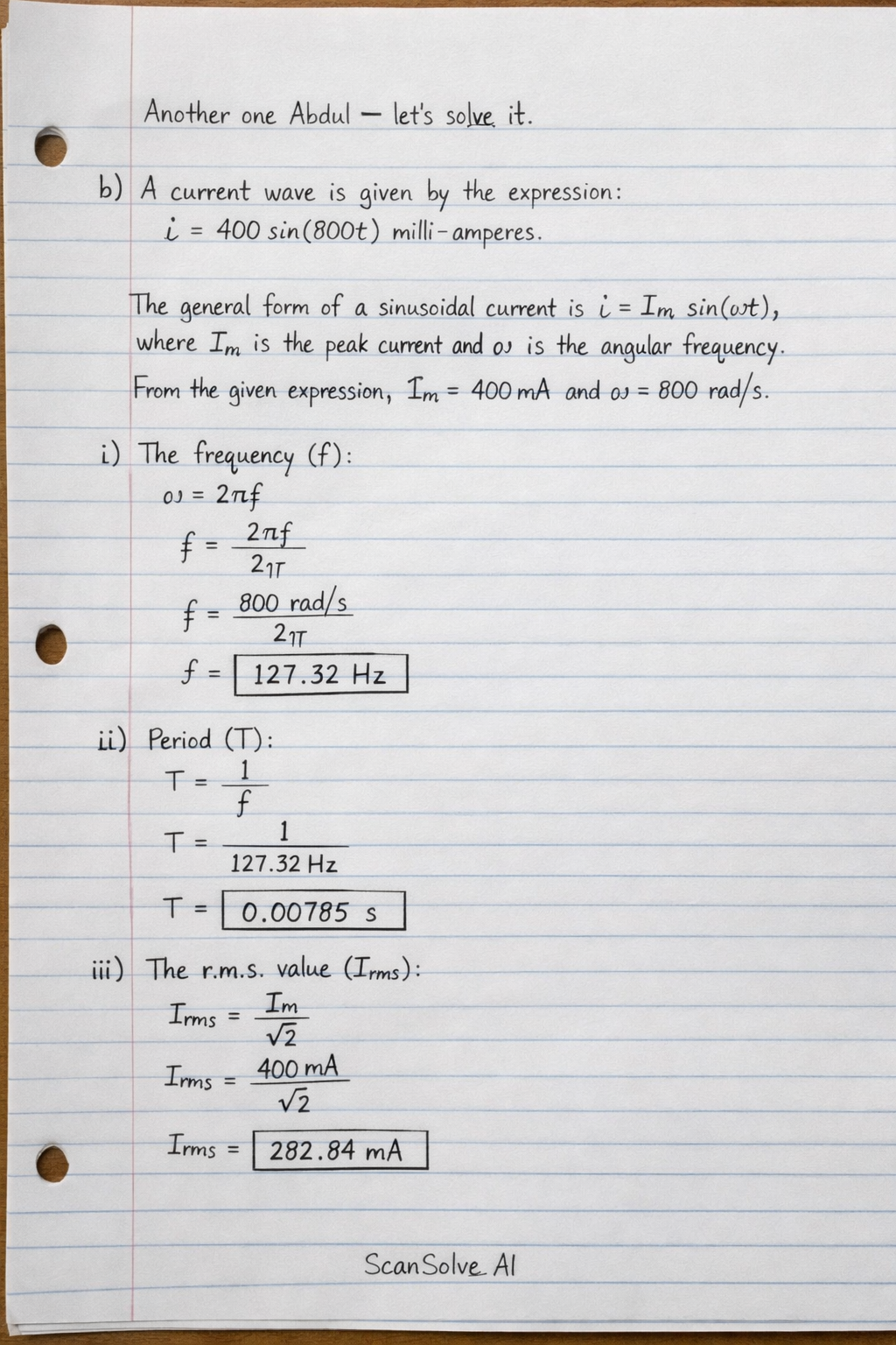
A current wave is given by the expression i = 400sin(800t) milli-amperes. Calculate: (i) The frequency (ii)period (iii) the r.m.s value (iv) the time t when I = 250mA

The magnitude of the impedance is $|Z| = \sqrt{R^2 + X_L^2}$.

The phase angle of the impedance is $\phi = \arctan\left(\frac{X_L}{R}\right)$.

The magnitude of the current is $|I| = \frac{|V|}{|Z|}$.

The current lags the voltage because the load is inductive.

The power factor (PF) is $\cos(\phi)$.

ii) The value of the capacitor required across the load to improve the power factor to 0.95 lagging.

Initial power factor $PF_1 = 0.287$.
Initial phase angle $\phi_1 = 73.30^\circ$.
Active power $P = V I \cos(\phi_1) = 240\text{V} \times 4.60\text{A} \times 0.287 = 316.896\text{ W}$.
Alternatively, $P = I^2 R = (4.60\text{A})^2 \times 15\Omega = 21.16 \times 15\text{ W} = 317.4\text{ W}$. (Using $I=4.60$ for calculation)
Let's use $P = \frac{V^2 R}{|Z|^2} = \frac{240^2 \times 15}{2725} = \frac{57600 \times 15}{2725} = \frac{864000}{2725} \approx 317.0\text{ W}$.
Initial reactive power $Q_1 = V I \sin(\phi_1) = 240\text{V} \times 4.60\text{A} \times \sin(73.30^\circ) = 240\text{V} \times 4.60\text{A} \times 0.958 = 1057.6\text{ VAR}$.
Alternatively, $Q_1 = I^2 X_L = (4.60\text{A})^2 \times 50\Omega = 21.16 \times 50\text{ VAR} = 1058\text{ VAR}$.

Target power factor $PF_2 = 0.95$ lagging.

The active power $P$ remains the same.
Target reactive power $Q_2 = P \tan(\phi_2)$.

The capacitor provides leading reactive power, so it reduces the lagging reactive power.

The reactive power of a capacitor is $Q_c = \frac{V^2}{X_C} = V^2 \omega C$.
Angular frequency $\omega = 2\pi f = 2\pi \times 50\text{ Hz} = 100\pi\text{ rad/s}$.

3a. Give four (4) comparisons between magnetic circuit and electric circuit.

• Driving Force: In an electric circuit, the driving force is the electromotive force (EMF), measured in Volts. In a magnetic circuit, it is the magnetomotive force (MMF), measured in Ampere-turns.
• Flow: In an electric circuit, the flow is electric current (charge carriers), measured in Amperes. In a magnetic circuit, the flow is magnetic flux, measured in Webers.
• Opposition to Flow: In an electric circuit, the opposition to current flow is resistance, measured in Ohms. In a magnetic circuit, the opposition to flux is reluctance, measured in Ampere-turns/Weber.
• Governing Laws: Electric circuits are governed by Ohm's Law ($V=IR$) and Kirchhoff's Laws. Magnetic circuits are governed by Hopkinson's Law (analogous to Ohm's Law for magnetic circuits, $MMF = \Phi S$).

3b. Derive the equation for the reluctance of a uniform magnetic material in terms of dimensions of the materials and other relevant parameters.

The magnetomotive force (MMF) is given by $MMF = NI$, where $N$ is the number of turns and $I$ is the current.
The magnetic flux ($\Phi$) is given by $\Phi = BA$, where $B$ is the magnetic flux density and $A$ is the cross-sectional area.

The magnetic flux density $B$ is related to the magnetic field strength $H$ by $B = \mu H$, where $\mu$ is the permeability of the material.
The permeability $\mu$ can also be expressed as $\mu = \mu_0 \mu_r$, where $\mu_0$ is the permeability of free space and $\mu_r$ is the relative permeability.
So, $B = \mu_0 \mu_r H$.

For a uniform magnetic circuit of length $l$, the magnetic field strength $H$ is given by $H = \frac{MMF}{l} = \frac{NI}{l}$.

Substitute the expression for $H$ into the equation for $B$:

Now substitute this expression for $B$ into the equation for $\Phi$:

Reluctance ($S$) is defined as the ratio of MMF to flux:

Substitute the expressions for MMF and $\Phi$:

Cancel $NI$ from the numerator and denominator:

Since $\mu = \mu_0 \mu_r$, the equation can also be written as:

Where $l$ is the length of the magnetic path, $A$ is the cross-sectional area, and $\mu$ is the absolute permeability of the material.

3c. A closed magnetic circuit is made of material of relative permeability 600, of length 40cm and having a cross-sectional area of $100\text{mm}^2$. A 400-turn coil is wound on the magnetic core. The coil carries a current of $500\text{mA}$.

Given:
Relative permeability $\mu_r = 600$
Length $l = 40\text{cm} = 0.4\text{m}$
Cross-sectional area $A = 100\text{mm}^2 = 100 \times (10^{-3}\text{m})^2 = 100 \times 10^{-6}\text{m}^2 = 10^{-4}\text{m}^2$
Number of turns $N = 400$
Current $I = 500\text{mA} = 0.5\text{A}$
Permeability of free space $\mu_0 = 4\pi \times 10^{-7}\text{ H/m}$

i) The reluctance of the magnetic circuit ($S$)

ii) The flux set up in the core ($\Phi$)

iii) The magneto motive force (MMF)

IV) The inductance of the magnetic circuit ($L$)
The inductance $L$ can be calculated using the formula $L = \frac{N^2}{S}$.

4a. Define the term resonance as applied to ac circuits. Sketch a resonance curve as applied to RC circuits and hence deduce the equation for resonant frequency.

• Definition of Resonance: Resonance in an AC circuit is a condition that occurs when the inductive reactance ($X_L$) and capacitive reactance ($X_C$) are equal in magnitude, effectively canceling each other out. This leads to the circuit's impedance being purely resistive, resulting in maximum current (in series RLC circuits) or maximum voltage (in parallel RLC circuits) at a specific frequency called the resonant frequency.

• Sketch a resonance curve as applied to RC circuits: The question asks for a resonance curve for RC circuits. However, resonance, in the sense of $X_L = X_C$, does not occur in a simple RC circuit as it lacks an inductor. A resonance curve typically depicts the current or voltage response of an RLC circuit as frequency varies, showing a peak at the resonant frequency. If the question implies a series RLC circuit, the curve would look like this: (Imagine a graph with "Current (I)" on the y-axis and "Frequency (f)" on the x-axis. The curve starts low, rises to a distinct peak at a specific frequency (the resonant frequency $f_0$), and then falls back down.)

• Deduce the equation for resonant frequency: For a series RLC circuit, resonance occurs when the inductive reactance equals the capacitive reactance:

  $$X_L = X_C$$

  We know that $X_L = \omega L$ and $X_C = \frac{1}{\omega C}$, where $\omega = 2\pi f$.

  $$\omega L = \frac{1}{\omega C}$$

  Multiply both sides by $\omega$:

  $$\omega^2 L = \frac{1}{C}$$ $$\omega^2 = \frac{1}{LC}$$

  Take the square root of both sides:

  $$\omega = \frac{1}{\sqrt{LC}}$$

  Substitute $\omega = 2\pi f_0$ (where $f_0$ is the resonant frequency):

  $$2\pi f_0 = \frac{1}{\sqrt{LC}}$$

  Solve for $f_0$:

  $$f_0 = \boxed{\frac{1}{2\pi\sqrt{LC}}}$$

4b. In the figure drawn below, the circuit is at resonant at a frequency of 490Hz.
The circuit consists of an $8\Omega$ resistor, a $50\text{mH}$ inductor, and a capacitor C in series with a $10\text{V}$ source.

Given:
Resonant frequency $f_0 = 490\text{Hz}$
Resistance $R = 8\Omega$
Inductance $L = 50\text{mH} = 0.05\text{H}$
Voltage $V = 10\text{V}$ (RMS)

i. Current at resonance ($I_0$)
At resonance, the impedance of a series RLC circuit is purely resistive, meaning $Z = R$.

ii. Value of C
At resonance, $f_0 = \frac{1}{2\pi\sqrt{LC}}$. We can rearrange this to solve for C.

iii. Capacitor voltage at resonance ($V_C$)
First, calculate the capacitive reactance $X_C$ at resonance.

Now, calculate the capacitor voltage:

iv. Inductor voltage at resonance ($V_L$)
First, calculate the inductive reactance $X_L$ at resonance.

Now, calculate the inductor voltage:

(Note: $V_L$ and $V_C$ should be equal at resonance, the slight difference is due to rounding in intermediate steps.)

v. Quality factor of the circuit ($Q$)
For a series RLC circuit, the quality factor is $Q = \frac{X_L}{R}$ (or $\frac{X_C}{R}$).

vi. Bandwidth of the circuit (BW)
The bandwidth of a series RLC circuit is given by $BW = \frac{f_0}{Q}$.

7a. Draw the circuit diagram of a 3-phase, 4-wire power system feeding a delta-connected load, show all relevant currents in the circuit.

(Imagine a diagram with the following elements and connections)

• Source Side:
  • Three phase lines labeled R, Y, B.
  • A neutral line labeled N.
  • The source could be represented as three voltage sources (e.g., star-connected) providing phase voltages $V_{RN}, V_{YN}, V_{BN}$ and line voltages $V_{RY}, V_{YB}, V_{BR}$.
• Load Side (Delta-connected):
  • Three impedances $Z_{RY}$, $Z_{YB}$, $Z_{BR}$ connected in a triangle (delta) configuration.
  • $Z_{RY}$ connected between R and Y lines.
  • $Z_{YB}$ connected between Y and B lines.
  • $Z_{BR}$ connected between B and R lines.
• Currents:
  • Line Currents: $I_R$, $I_Y$, $I_B$ flowing from the source lines to the load connection points.
  • Phase Currents: $I_{RY}$ (flowing through $Z_{RY}$), $I_{YB}$ (flowing through $Z_{YB}$), $I_{BR}$ (flowing through $Z_{BR}$).
  • Neutral Current: $I_N$ (flowing in the neutral line). For a delta load, the neutral line is typically not connected to the load directly, so $I_N$ would be zero unless there's an imbalance in the source or other connections. However, if the question implies a 4-wire system feeding the delta load, it means the 4 wires are available, but only 3 are used for the delta load.

Diagram Description:
Draw three vertical lines (R, Y, B) representing the phase conductors, and one more vertical line (N) for the neutral.
Connect the R, Y, B lines to the corners of a triangle formed by three impedances.

• Connect $Z_{RY}$ between R and Y.
• Connect $Z_{YB}$ between Y and B.
• Connect $Z_{BR}$ between B and R. Show arrows for line currents $I_R$, $I_Y$, $I_B$ entering the delta load from the respective phase lines. Show arrows for phase currents $I_{RY}$, $I_{YB}$, $I_{BR}$ flowing within the delta impedances. (For a balanced delta load, $I_L = \sqrt{3} I_P$ and $V_L = V_P$).

7b. A star-connected load having the following impedances, $Z_r = (20 - j16)\Omega$, $Z_y = (16 - j20)\Omega$ and $Z_b = (20 - j0)\Omega$ are connected across a 3-phase, 4-wire system having a line voltage of 420V.

Given:
$Z_r = (20 - j16)\Omega$
$Z_y = (16 - j20)\Omega$
$Z_b = (20 - j0)\Omega$ (purely resistive)
Line voltage $V_L = 420\text{V}$
3-phase, 4-wire system.

i) Draw the circuit diagram

(Imagine a diagram with the following elements and connections)

• Source Side:
  • Three phase lines labeled R, Y, B.
  • A neutral line labeled N.
  • The source could be represented as three voltage sources (e.g., star-connected) providing phase voltages $V_{RN}, V_{YN}, V_{BN}$ and line voltages $V_{RY}, V_{YB}, V_{BR}$.
• Load Side (Star-connected):
  • Three impedances $Z_r$, $Z_y$, $Z_b$ connected from each phase line to a common neutral point (N').
  • $Z_r$ connected between R line and N'.
  • $Z_y$ connected between Y line and N'.
  • $Z_b$ connected between B line and N'.
  • The load neutral point N' is connected to the system neutral line N.
• Currents and Voltages:
  • Line Currents: $I_R$, $I_Y$, $I_B$ flowing from the source lines through the respective impedances. In a star connection, line currents are equal to phase currents.
  • Phase Voltages: $V_{RN'}$, $V_{YN'}$, $V_{BN'}$ across each impedance.
  • Neutral Current: $I_N$ flowing in the neutral line, which will be non-zero because the load is unbalanced ($Z_r \neq Z_y \neq Z_b$).

Diagram Description:
Draw three vertical lines (R, Y, B) representing the phase conductors, and one more vertical line (N) for the neutral.
Draw a central point N' (load neutral).
Connect $Z_r$ between R and N'.
Connect $Z_y$ between Y and N'.
Connect $Z_b$ between B and N'.
Connect N' to N.
Show arrows for line currents $I_R$, $I_Y$, $I_B$ flowing from the phase lines through the impedances towards N'.
Show an arrow for neutral current $I_N$ flowing in the neutral line.
Show phase voltages $V_{RN'}$, $V_{YN'}$, $V_{BN'}$ across each impedance.
(For a star connection, $V_P = V_L / \sqrt{3}$ and $I_L = I_P$).