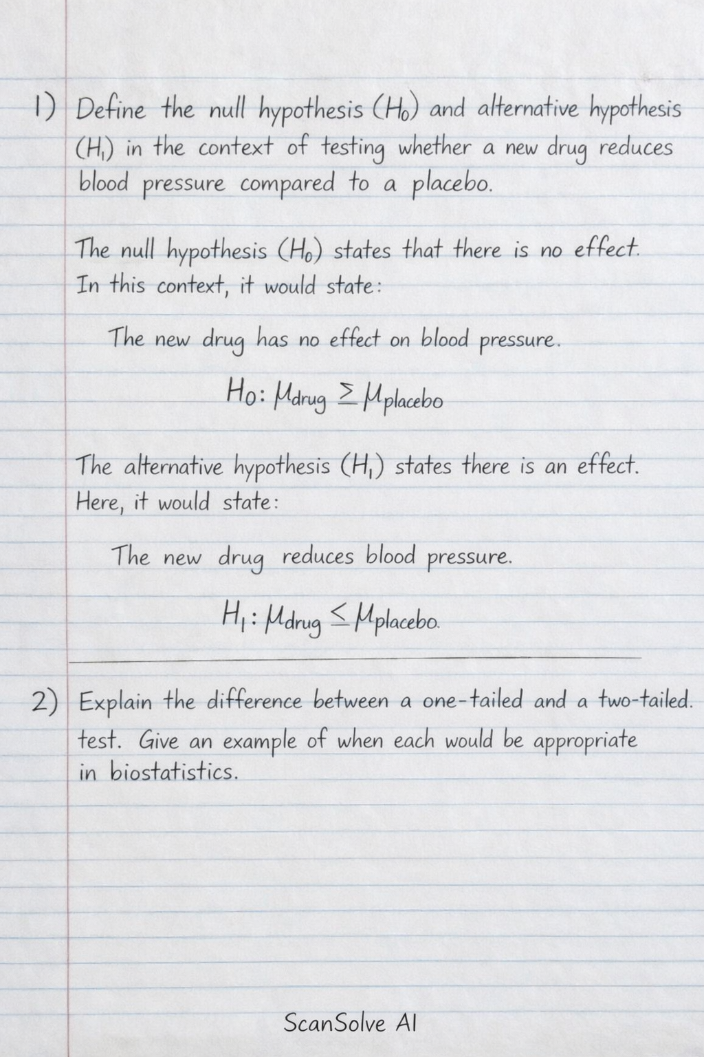
Here are the answers to your questions: 1. Define the null hypothesis (H₀) and alternative hypothesis (H₁) in the context of testing whether a new drug reduces blood pressure compared to a placebo. The null hypothesis* (H₀) states that there is no difference or no effect. In this context, it would state that the new drug has no effect on blood pressure, meaning the mean blood pressure of patients taking the drug is the same as or higher than those taking a placebo. $$H_0: \mu_{\text{drug}} \ge \mu_{\text{placebo}}$$ The alternative hypothesis (H₁) states that there is a significant difference or an effect. Here, it would state that the new drug reduces* blood pressure, meaning the mean blood pressure of patients taking the drug is lower than those taking a placebo. $$H_1: \mu_{\text{drug}} < \mu_{\text{placebo}}$$ 2. Explain the difference between a one-tailed and a two-tailed test. Give an example of when each would be appropriate in biostatistics. A one-tailed test* (or directional test) is used when the alternative hypothesis specifies a direction for the effect (e.g., greater than or less than). The critical region for rejecting the null hypothesis is entirely in one tail of the sampling distribution. Example: Testing if a new drug reduces* blood pressure (as in question 1). A two-tailed test* (or non-directional test) is used when the alternative hypothesis states that there is a difference, but does not specify the direction (e.g., simply "different from"). The critical region is split between both tails of the sampling distribution. Example: Testing if the mean cholesterol level of a new diet group is different* from the mean cholesterol level of a control group (it could be higher or lower). 3. What is a Type I error? What is a Type II error? Provide a medical example of each. A Type I error* occurs when the null hypothesis is true, but we incorrectly reject it. It is a "false positive." Medical example:* Concluding that a new drug is effective in treating a disease when, in reality, it has no effect. A Type II error* occurs when the null hypothesis is false, but we incorrectly fail to reject it. It is a "false negative." Medical example: Concluding that a new drug is not effective in treating a disease when, in reality, it is* effective. 4. Why is the p-value not the probability that the null hypothesis is true? The p-value is the probability of observing data as extreme as, or more extreme than, the data observed, assuming that the null hypothesis is true. It does not tell us the probability that the null hypothesis is true or false. The null hypothesis is either true or false; it's not a random variable. The p-value quantifies the strength of evidence against the null hypothesis, not the probability of its truth. --- Computational Questions 1. A study tests whether the mean hemoglobin level in a population is 12 g/dL. A sample of 40 patients has a mean of 11.6 g/dL and a standard deviation of 1.2 g/dL. State the hypotheses. Null Hypothesis ($H_0$): The mean hemoglobin level in the population is 12 g/dL. $$H_0: \mu = 12 \text{ g/dL}$$ Alternative Hypothesis ($H_1$): The mean hemoglobin level in the population is not 12 g/dL. $$H_1: \mu \ne 12 \text{ g/dL}$$ Conduct a one-sample t-test at \(\alpha = 0.05\). Step 1: Identify the given values. Population mean ($\mu_0$) = 12 g/dL Sample mean ($\bar{x}$) = 11.6 g/dL Sample standard deviation ($s$) = 1.2 g/dL Sample size ($n$) = 40 Significance level ($\alpha$) = 0.05 Step 2: Calculate the standard error of the mean ($SE$). $$SE = \frac{s}{\sqrt{n}}$$ $$SE = \frac{1.2}{\sqrt{40}}$$ $$SE = \frac{1.2}{6.3246}$$ $$SE \approx 0.1897$$ Step 3: Calculate the t-statistic. $$t = \frac{\bar{x} - \mu_0}{SE}$$ $$t = \frac{11.6 - 12}{0.1897}$$ $$t = \frac{-0.4}{0.1897}$$ $$t \approx -2.108$$ Step 4: Determine the degrees of freedom ($df$). $$df = n - 1 = 40 - 1 = 39$$ Step 5: Find the critical t-values for a two-tailed test at $\alpha = 0.05$ with $df = 39$. Using a t-distribution table or calculator, the critical t-values are approximately $\pm 2.023$. Step 6: Make a decision. Since the calculated t-statistic ($-2.108$) is less than the lower critical t-value ($-2.023$), it falls into the rejection region. $$\boxed{\text{Reject the null hypothesis.}}$$ Interpret the result. Since the null hypothesis is rejected, there is sufficient evidence at the $\alpha = 0.05$ significance level to conclude that the mean hemoglobin level in the population is significantly different from 12 g/dL. 2. Researchers compare recovery times between two groups: treatment (n=25, mean=8 days, SD=2) and control (n=30, mean=10 days, SD=2.5). Formulate hypotheses. Null Hypothesis ($H_0$): There is no difference in mean recovery times between the treatment and control groups. $$H_0: \mu_{\text{treatment}} = \mu_{\text{control}}$$ Alternative Hypothesis ($H_1$): The treatment group has a significantly shorter recovery time than the control group. (This implies a one-tailed test, as the question asks if treatment reduces* recovery time). $$H_1: \mu_{\text{treatment}} < \mu_{\text{control}}$$ Perform a two-sample t-test. (Assuming unequal variances due to different standard deviations and sample sizes, using Welch's t-test approach for the t-statistic calculation). Step 1: Identify the given values. Treatment group 1: $n_1 = 25$, $\bar{x}_1 = 8$, $s_1 = 2$ Control group 2: $n_2 = 30$, $\bar{x}_2 = 10$, $s_2 = 2.5$ Step 2: Calculate the standard error for the difference between means. $$SE_{\bar{x}_1 - \bar{x}_2} = \sqrt{\frac{s_1^2}{n_1} + \frac{s_2^2}{n_2}}$$ $$SE_{\bar{x}_1 - \bar{x}_2} = \sqrt{\frac{2^2}{25} + \frac{2.5^2}{30}}$$ $$SE_{\bar{x}_1 - \bar{x}_2} = \sqrt{\frac{4}{25} + \frac{6.25}{30}}$$ $$SE_{\bar{x}_1 - \bar{x}_2} = \sqrt{0.16 + 0.20833}$$ $$SE_{\bar{x}_1 - \bar{x}_2} = \sqrt{0.36833}$$ $$SE_{\bar{x}_1 - \bar{x}_2} \approx 0.6069$$ Step 3: Calculate the t-statistic. $$t = \frac{(\bar{x}_1 - \bar{x}_2) - (\mu_1 - \mu_2)}{SE_{\bar{x}_1 - \bar{x}_2}}$$ Under the null hypothesis, $\mu_1 - \mu_2 = 0$. $$t = \frac{8 - 10}{0.6069}$$ $$t = \frac{-2}{0.6069}$$ $$t \approx -3.295$$ Step 4: Determine the degrees of freedom (Welch-Satterthwaite equation is complex; for practical purposes, software is used. A conservative estimate is $df = \min(n_1-1, n_2-1) = \min(24, 29) = 24$). For a one-tailed test at $\alpha = 0.05$ with $df = 24$, the critical t-value is approximately $-1.711$. Step 5: Make a decision. Since the calculated t-statistic ($-3.295$) is less than the critical t-value ($-1.711$), it falls into the rejection region. $$\boxed{\text{Reject the null hypothesis.}}$$ State whether the treatment significantly reduces recovery time. $$\boxed{\text{Yes, the treatment significantly reduces recovery time.}}$$ --- Applied Scenario Questions 1. A clinical trial tests whether a vaccine prevents infection. Out of 200 vaccinated individuals, 10 became infected; out of 200 unvaccinated individuals, 30 became infected. Which statistical test should be used? Since we are comparing proportions of categorical outcomes (infected/not infected) between two independent groups (vaccinated/unvaccinated), a Chi-square test for independence or a Z-test for two proportions would be appropriate. The Chi-square test is generally more versatile for contingency tables. $$\boxed{\text{Chi-square test for independence}}$$ State the hypotheses. Null Hypothesis ($H_0$): There is no association between vaccination status and infection status (i.e., the proportion of infected individuals is the same in both groups). $$H_0: P_{\text{infected|vaccinated}} = P_{\text{infected|unvaccinated}}$$ Alternative Hypothesis ($H_1$): There is an association between vaccination status and infection status (i.e., the proportion of infected individuals differs between the two groups). $$H_1: P_{\text{infected|vaccinated}} \ne P_{\text{infected|unvaccinated}}$$ Carry out the test and interpret the findings. Step 1: Create a contingency table of observed frequencies. | | Infected | Not Infected | Total | | :---------- | :-------- | :----------- | :---- | | Vaccinated | 10 | 190 | 200 | | Unvaccinated | 30 | 170 | 200 | | Total | 40 | 360 | 400 | Step 2: Calculate expected frequencies ($E_{ij} = \frac{\text{Row Total} \times \text{Column Total}}{\text{Grand Total}}$). $E_{\text{Vaccinated, Infected}} = \frac{200 \times 40}{400} = 20$ $E_{\text{Vaccinated, Not Infected}} = \frac{200 \times 360}{400} = 180$ $E_{\text{Unvaccinated, Infected}} = \frac{200 \times 40}{400} = 20$ $E_{\text{Unvaccinated, Not Infected}} = \frac{200 \times 360}{400} = 180$ Step 3: Calculate the Chi-square statistic ($\chi^2 = \sum \frac{(O_{ij} - E_{ij})^2}{E_{ij}}$). $$\chi^2 = \frac{(10-20)^2}{20} + \frac{(190-180)^2}{180} + \frac{(30-20)^2}{20} + \frac{(170-180