Show that for a delta-star transformation, Z1 = ZAZB/ZA+ZB+ZC, Z2 = ZBZC/ZA+ZB+ZC and Z3 = ZAZC/ZA+ZB+ZC. For the network shown in the diagram below, determine: i) the current flowing in the (0 + j10)Ω impedance

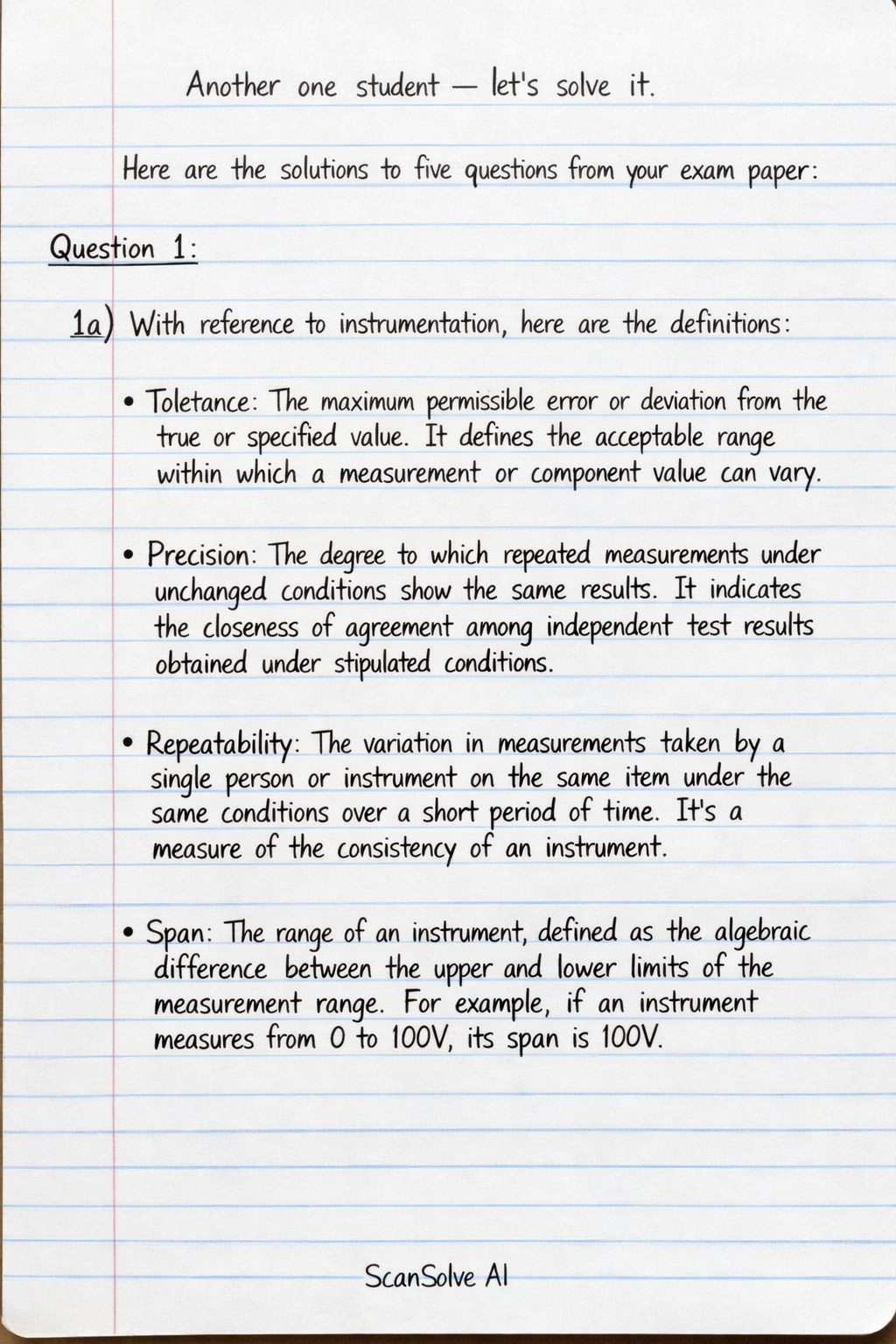
1a) With reference to instrumentation, here are the definitions:

• Tolerance: The maximum permissible error or deviation from the true or specified value. It defines the acceptable range within which a measurement or component value can vary.
• Precision: The degree to which repeated measurements under unchanged conditions show the same results. It indicates the closeness of agreement among independent test results obtained under stipulated conditions.
• Repeatability: The variation in measurements taken by a single person or instrument on the same item under the same conditions over a short period of time. It's a measure of the consistency of an instrument.
• Span: The range of an instrument, defined as the algebraic difference between the upper and lower limits of the measurement range. For example, if an instrument measures from 0 to 100V, its span is 100V.
• Linearity: The extent to which the output of an instrument is directly proportional to the input over its entire measurement range. A perfectly linear instrument would have a straight-line relationship between input and output.

1b) Here are the advantages and disadvantages of null and deflection types of measuring instruments:

• Null-type instruments:
  • Advantages: High accuracy, independent of indicating device calibration, less susceptible to parameter changes, often more sensitive.
  • Disadvantages: Slower response time, more complex to operate, cannot be used for rapidly changing quantities, often more expensive.
• Deflection-type instruments:
  • Advantages: Faster response time (direct readings), simpler to operate, can be used for rapidly changing quantities, generally less expensive.
  • Disadvantages: Lower accuracy (depends on scale calibration), more susceptible to errors from friction, temperature, and aging, can have a loading effect on the circuit.

1c) Null-type instruments are mainly used for high-precision measurements where accuracy is paramount, such as in laboratories, calibration standards, and industrial process control systems. They are preferred because they operate by balancing the unknown quantity against a known standard, meaning the measurement is taken when the detector indicates zero (null). This eliminates errors associated with the detector's calibration or non-linearity, making them inherently more accurate and reliable for precise work.

2a) Here is the difference between systematic and random errors:

• Systematic errors are consistent, repeatable errors inherent in the measurement system or method, causing measurements to consistently deviate from the true value in the same direction. They can often be identified and corrected.
• Random errors are unpredictable, variable errors due to uncontrollable fluctuations in the measurement process, causing measurements to vary randomly around the true value. They cannot be eliminated but can be minimized by taking multiple measurements and averaging.

2b) Here are the typical sources of these two types of error:

• Sources of Systematic Errors: Instrumental errors (faulty calibration, zero error), environmental errors (consistent external influences), observational errors (parallax), theoretical errors (model approximations).
• Sources of Random Errors: Environmental fluctuations (unpredictable changes), human limitations (estimation, reaction time), instrument limitations (noise, resolution), variations in the measured quantity itself.

2c) To calculate the value of density and its possible error:
Given: $a = 100\text{mm} \pm 1\%$, $b = 200\text{mm} \pm 1\%$, $c = 300\text{mm} \pm 1\%$, $m = 20\text{kg} \pm 0.5\%$.
Density $\rho = \frac{m}{V}$, where $V = a \times b \times c$.

3a) All analogue electrical indicating instruments require three essential devices:

1. Deflecting System: This system produces a deflecting torque that causes the pointer to move away from its zero position, proportional to the measured quantity.
2. Controlling System: This system provides a controlling torque that opposes the deflecting torque, ensuring the pointer comes to rest at a specific position corresponding to the measured quantity.
3. Damping System: This system prevents the pointer from oscillating excessively around its final steady position, bringing it to rest quickly to allow for easy reading.

3b) To calculate the value of the shunt:
Given: $I_m = 40\text{ mA} = 0.04\text{ A}$, $R_m = 25\Omega$, $I = 50\text{ A}$.

Given: $f_0 = 1.2\text{ kHz} = 1200\text{ Hz}$, $Q = 30$, $Z_0 = 50\Omega$.
At resonance, $Z_0 = R$, so $R = 50\Omega$.

5a) The circuit diagram to measure 3-phase power using the two-wattmeter method involves connecting two wattmeters to the three-phase supply and load.

• Wattmeter 1 (W1): Its current coil is connected in series with line L1. Its voltage coil is connected between line L1 and line L2.
• Wattmeter 2 (W2): Its current coil is connected in series with line L3. Its voltage coil is connected between line L3 and line L2. Line L2 serves as the common potential point for the voltage coils of both wattmeters.

5b) To derive the equation for the power output and power angle from the two-wattmeter readings:
Let $W_1$ and $W_2$ be the readings of the two wattmeters. For a balanced 3-phase load, the readings are given by:

where $V_L$ is the line voltage, $I_L$ is the line current, and $\phi$ is the phase angle of the load.